
Article
Building a methylene blue calibration curve: blanks, range, and linearity
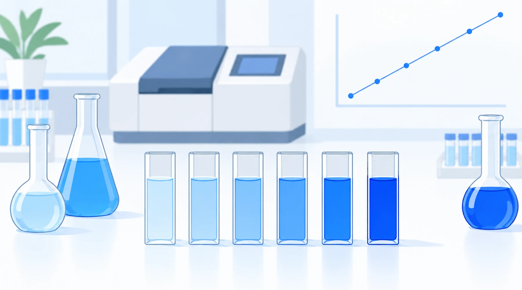
Two analysts share one stock bottle of methylene blue and each builds a calibration curve. The first gets a straight line through the origin and measures unknowns with confidence. The second gets a line that bends at the top, an intercept that will not close to zero, and sample results that drift with dilution. Same dye, same instrument, same wavelength. The difference is not skill. It is design: what went into the blank, which concentrations were chosen, and whether the checked range stayed inside the region where one simple model still holds.
A calibration curve is a contract between an instrument response and a concentration, valid only under the conditions in which it was built. For methylene blue that contract has a known weak point. The dye self-associates in water, so the absorbing species changes with concentration. A curve built across that change will not be straight, and no amount of statistics will fix it. This article shows how to design the curve so the line means something: pick the right blank, hold the range inside the monomer regime, replicate honestly, and read curvature as information rather than noise.
Start with the blank, not the standards
The blank defines zero, and for methylene blue it must contain everything except the dye. Same water grade, same buffer and pH, same salts, same cosolvent fraction, same temperature. Prepare the calibrants in that identical matrix. The reason is chemical, not bureaucratic. Salt and solvent shift the balance between monomer, dimer, and higher aggregates, which changes the spectrum at the measuring wavelength. A water-only blank cannot correct a matrix-induced change in speciation. The global analysis of methylene blue spectra in water, available through its open access record, varied sodium chloride from 0 to 0.15 M precisely because ionic strength moves the equilibrium, and aggregation increased with salt.
One practical consequence: never calibrate in deionized water and then measure samples in phosphate buffer or wastewater filtrate. When no analyte-free matrix exists, standard addition into the sample itself beats an unmatched external curve. Related guidance on keeping aqueous assays honest lives in the matrix and interference discussion, and the general principles of quantitative dye assays are covered in the assay design overview.
Choose a range where one species dominates
Quantification at the long wavelength band near 664 nm assumes most of the dye is monomeric. In plain water that assumption holds only while solutions stay dilute, roughly in the low micromolar region. Published empirical slopes illustrate the boundary: calibrations kept below about 7 micromolar in 1 cm cells give a slope near 82,000 M-1 cm-1, while a calibration stretched up to about 37 micromolar drops to roughly 67,100 because the upper standards already contain appreciable dimer. Every coefficient cited here is condition-labeled in the spectral reference for methylene blue, which is the right place to compare numbers; this article uses them only to set the range.
The design rules follow directly:
- Keep the top standard dilute enough that the spectrum shape is stable. During development, scan the full visible range (about 550 to 750 nm) for each level instead of reading one wavelength. If normalized spectra change shape with concentration, the chemistry is changing and the range is too wide.
- Track the ratio of absorbance near 610 nm to absorbance near 665 nm across levels. A ratio that climbs with concentration means the dimer shoulder is growing and the monomer model is failing. This diagnostic is explained further in the aggregation and concentration effects guide.
- Use a 1 cm cell for low micromolar work. With a slope near 82,000, 5 micromolar gives absorbance near 0.41 and 10 micromolar gives about 0.82, both comfortable for most instruments.
- For concentrated stocks, shorten the path instead of accepting absorbance far above 1, but remember that a short path fixes the photometry, not the chemistry. Aggregation depends on concentration, not path length, so a concentrated stock still needs its own speciation-aware treatment rather than a dilute monomer curve.
The global fit behind much of this picture covered 224 spectra from 1.1 micromolar to 3.4 millimolar and found tetramer signal already detectable below 34 micromolar. That finding sets the mood: the linear window is narrower than intuition suggests, so verify it rather than assuming it.
Levels, replicates, and order
A curve with three points proves nothing. Validation guidance in ICH Q2(R2) asks for at least five concentrations to assess linearity, and six to eight nonzero levels give a more convincing working curve, especially near the top where aggregation begins. Space levels to cover the intended sample range with extra density where curvature is most likely, not in a geometric series chosen for convenience.
Measure each level in duplicate or triplicate, prepared independently rather than read three times from one flask. Independent replicates expose preparation error; repeat readings of one flask only expose instrument noise. The 2020 global study measured each solution three times, which remains a sound default. Randomize the reading order so that drift, adsorption to glass, or temperature change cannot masquerade as curvature. A quartz cuvette study found about 3 percent of dye adsorbing from a 34 micromolar solution within 10 minutes, so keep contact time, cuvette, cleaning, and sequence consistent across the run.
Illustrative worked example (not measured data)
The numbers below are invented to show the arithmetic. They are not laboratory measurements and must not be cited as methylene blue data. What matters is the pattern of checks around them.
Suppose six standards in matched buffer, 1 cm path, read at 665 nm against the matched blank:
| Level | Nominal conc. (µM) | A665 rep 1 | A665 rep 2 | Mean A665 | A610/A665 |
|---|---|---|---|---|---|
| S1 | 0 (blank) | 0.000 | 0.001 | 0.001 | not defined |
| S2 | 1.0 | 0.083 | 0.081 | 0.082 | 0.42 |
| S3 | 2.0 | 0.165 | 0.163 | 0.164 | 0.42 |
| S4 | 3.5 | 0.287 | 0.285 | 0.286 | 0.43 |
| S5 | 5.0 | 0.408 | 0.410 | 0.409 | 0.43 |
| S6 | 7.0 | 0.562 | 0.566 | 0.564 | 0.46 |
A straight-line fit of mean absorbance against concentration gives a slope near 0.0805 absorbance units per micromolar and an intercept within a few milliabsorbance units of zero. Dividing the slope by the path length converts it to an apparent absorptivity: 0.0805 per micromolar equals about 80,500 M-1 cm-1, consistent with a monomer-dominated interval in water. The checks that matter are not the R squared, which will look excellent either way. They are the near-zero intercept, the flat A610/A665 ratio across S2 through S5, and residuals scattered without a trend. The uptick in the ratio at S6 is the honest signal to either drop that level or flag 7 micromolar as the provisional top of this matrix and instrument combination.
An unknown read at 0.245 under identical conditions converts directly: 0.245 divided by 0.0805 per micromolar gives about 3.0 micromolar, before any sample dilution factor is applied. Report the result with its conditions: wavelength, path, blank matrix, calibration interval, and date.
Fillable calibration worksheet
Copy this template into the lab record for each new matrix. One matrix, one sheet, one curve.
| Field | Entry |
|---|---|
| Matrix (water grade, buffer, salts, cosolvent) | |
| Reagent form and molar mass used (anhydrous vs hydrate) | |
| Stock preparation (mass, volume, date) | |
| Wavelength and spectral window scanned | |
| Path length and cuvette ID | |
| Blank absorbance at measuring wavelength | |
| Levels (nominal concentrations) | |
| Replicates per level (independent preparations) | |
| Reading order and contact time per cuvette | |
| Slope, intercept, residual pattern | |
| A610/A665 ratio across levels | |
| Accepted interval (lowest to highest standard kept) | |
| Unknown IDs, dilutions, and converted results |
The reagent-form row earns its place. Commercial methylene blue may be anhydrous salt or a hydrate such as the trihydrate, and the wrong molar mass silently biases every nominal concentration. Purity and specification checks for the starting material are covered in the quality and grade guide.
Verify with an independent check standard
A calibration curve should never grade its own homework. After fitting, prepare one check standard from a separately weighed stock, at a concentration near the middle of the accepted interval, and read it as an unknown. Agreement within a few percent confirms the preparation chain; a miss implicates the stock or the dilutions rather than the instrument. Repeat the check standard with each batch of samples. If it drifts while the curve is unchanged, suspect the working solutions or the cuvette before suspecting the samples. This single habit catches most of the quiet errors: a hydrate molar mass applied to an anhydrous bottle, a micropipette out of calibration, a buffer made up at the wrong ionic strength. Log the check recovery on the worksheet next to the slope, so a later reader can see that the line was tested, not just drawn.
Reading nonlinearity as a diagnosis
When the curve bends, the shape of the failure identifies the cause. Downward curvature at high absorbance with an unchanged spectral shape points at the instrument, often stray light biasing strong absorbances low. Curvature accompanied by a rising 610 nm shoulder points at the chemistry: dimer and higher aggregates absorbing differently from monomer. A blank that will not zero, or standards that fall over time, point at the container: adsorption to glass or cuvettes, especially if contact times varied down the run. And a clean line through points that still gives wrong sample results points at the matrix: samples differ from calibrants, so rebuild the curve in the sample matrix or switch to standard addition. Plot residuals against concentration in every case. A random scatter supports the straight-line model; a smile or frown refutes it more reliably than any R squared threshold, a point validation guidance endorses explicitly.
Methylene blue rewards this discipline. Its monomer band is strong, its chemistry is well mapped, and its failure modes announce themselves in the spectrum before they corrupt the numbers. Build the curve narrowly, blank it honestly, replicate it independently, and let the shape of the spectra vote on the range. The resulting line is short, but every point on it is true.
Illustrative calculations in this article use invented numbers to demonstrate method. Measured reference coefficients with full conditions appear in the linked spectral reference, and the underlying aggregation study is indexed at PMID 33251415.